Creating a site survey and developing a land management strategy
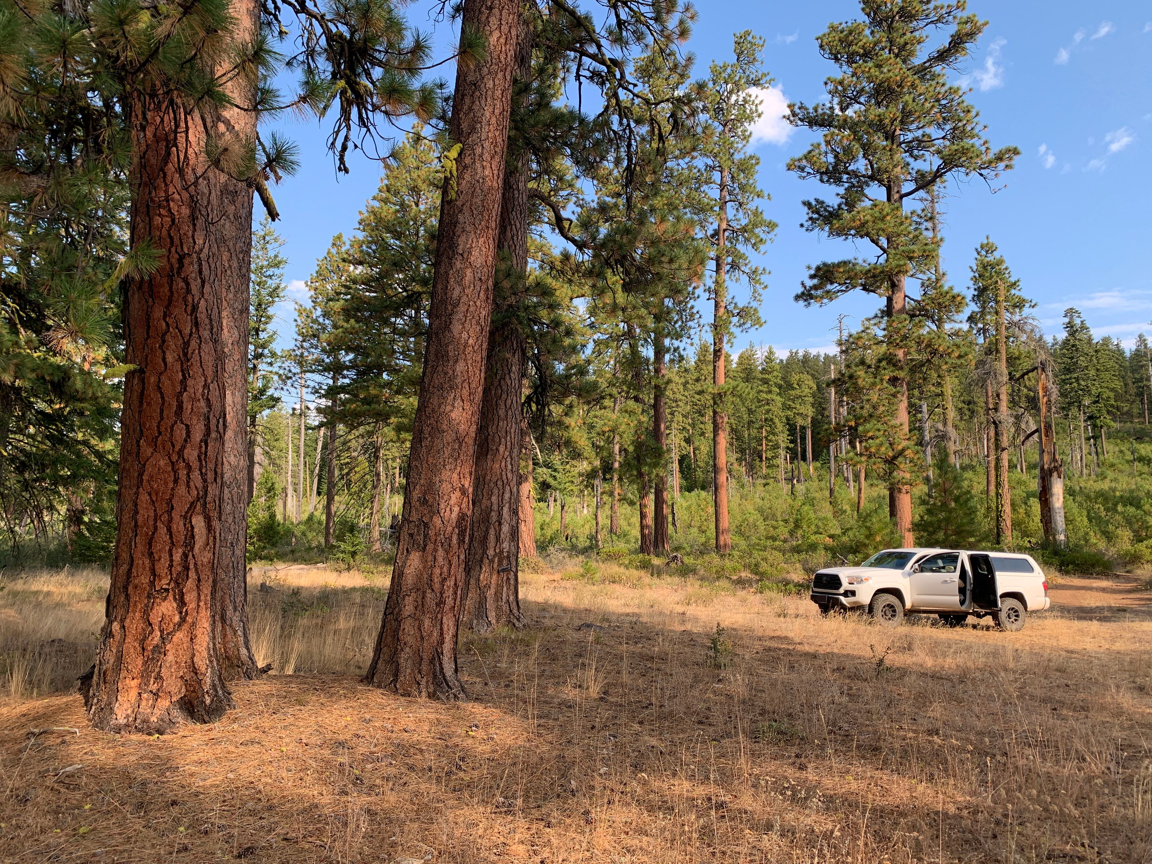
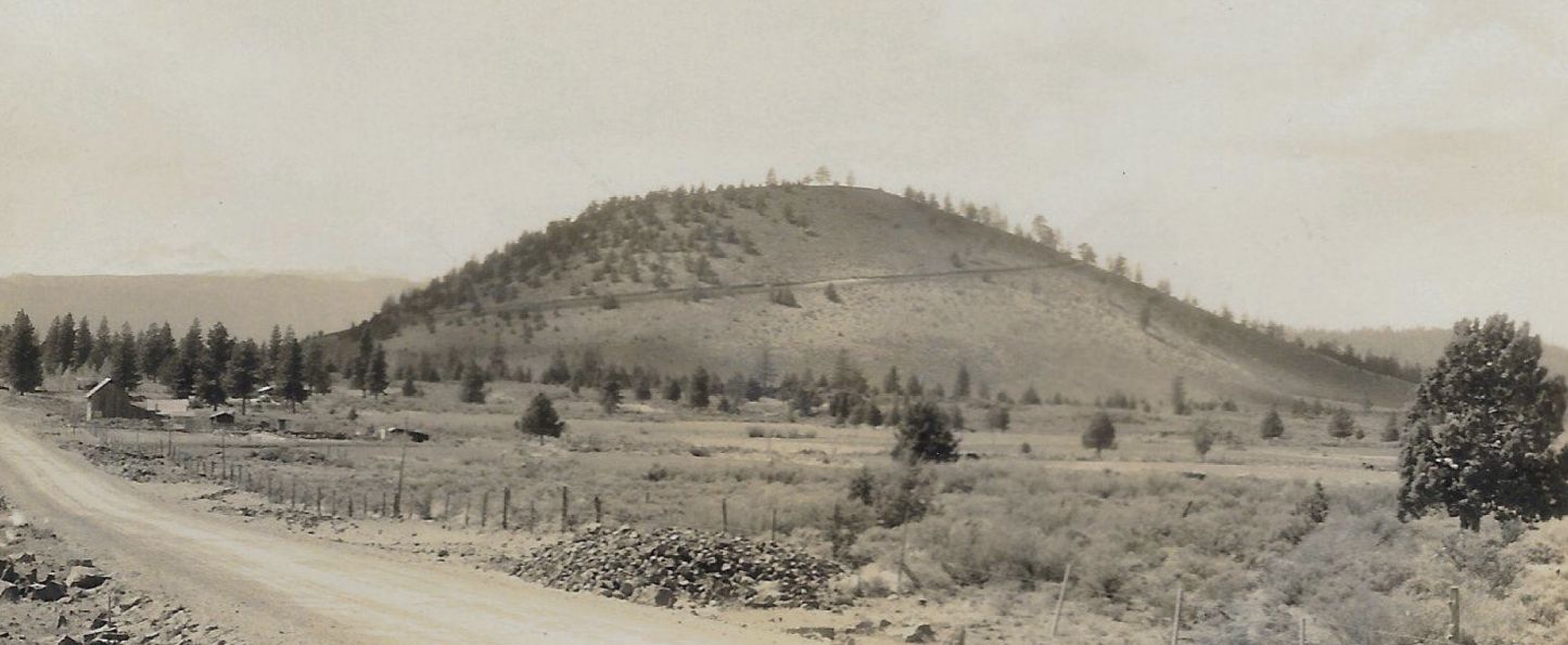
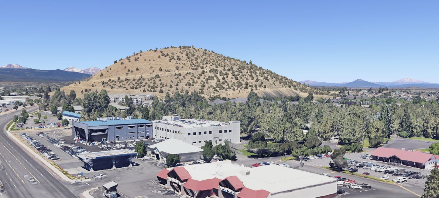
Our property is located in the transition zone where the the ponderosa pines that cover the eastern slopes of the Cascades gradually give way to western juniper and sagebrush. On the property there are two types of trees: mature (>80 yo) ponderosa pines (pinus ponderosa) and young (<50 yo) western junipers (juniperus occidentalis).
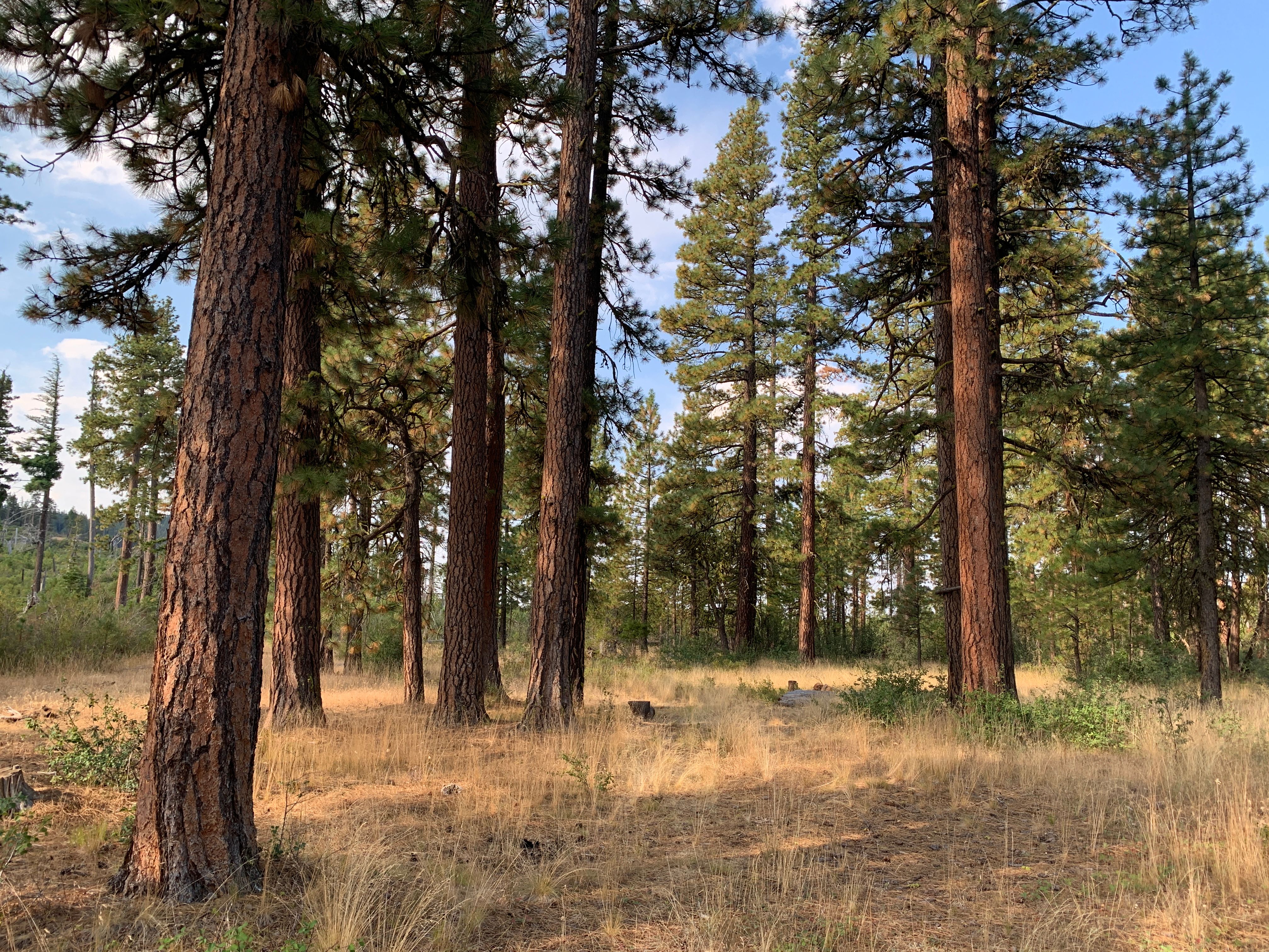
As we begin to install utilities, a driveway, and buildings, we’d like to keep the ponderosa pines undisturbed. They’re beautiful trees and take at least a human lifetime to get established. Old stands of ponderosa pines are lovely places to sit and spend an afternoon.
Juniper is taking over the world
Juniper, on the other hand, is less precious.
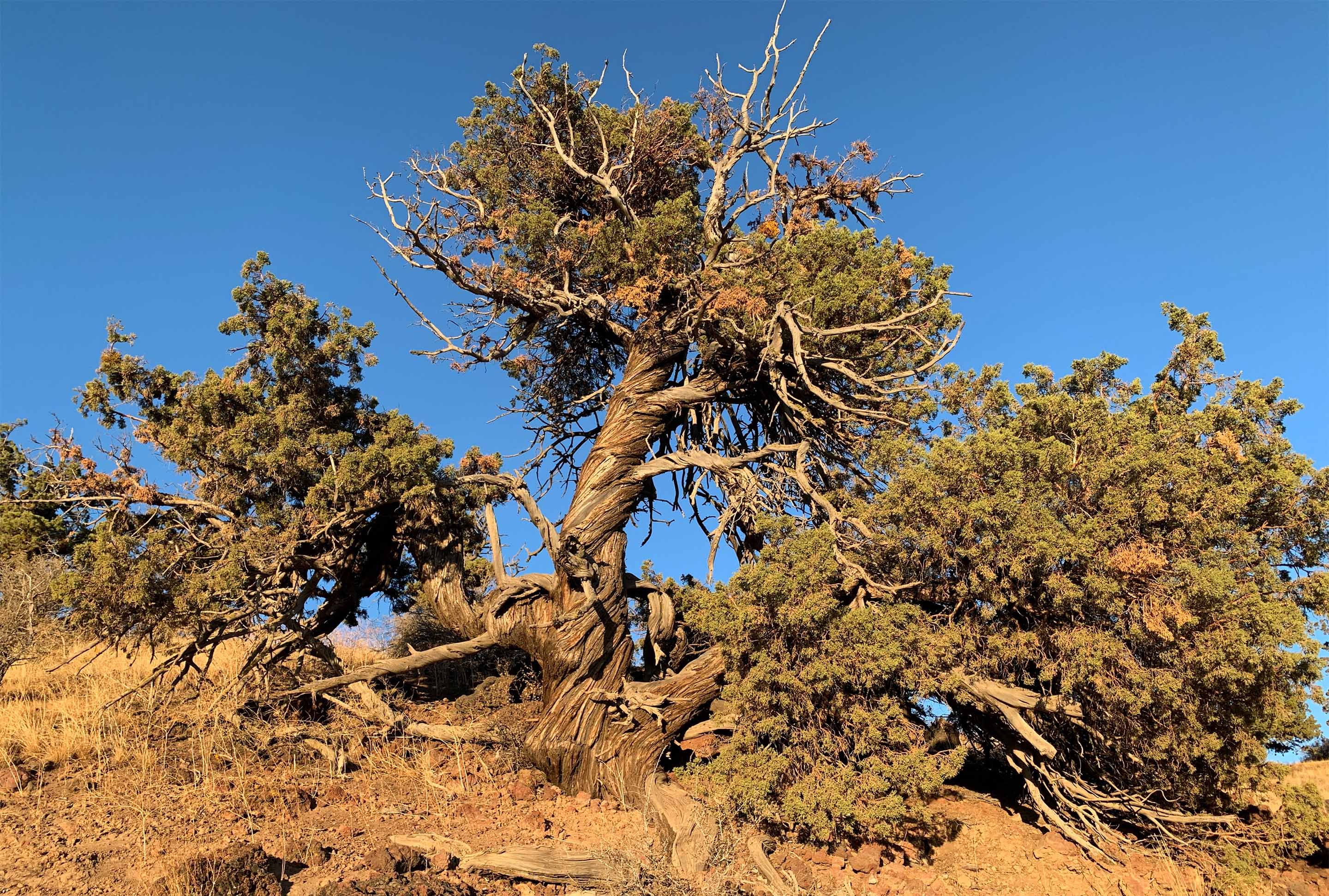
Western juniper is a common part of the central and eastern Oregon landscape. Junipers can live for over a thousand years and become gnarled and twisted old relics.
However, since western settlement began around 1870, juniper has been expanding beyond its range and taking over other ecosystems. I found this publication from OSU to be a nice summary of the situation.
The expansion is primarily because of the fire suppression that began in the early 1900’s. Lightning fires would have normally killed off young junipers before they reached maturity, leaving only the trees on rock outcroppings and isolated locations. Without fires, the junipers grow unencumbered.
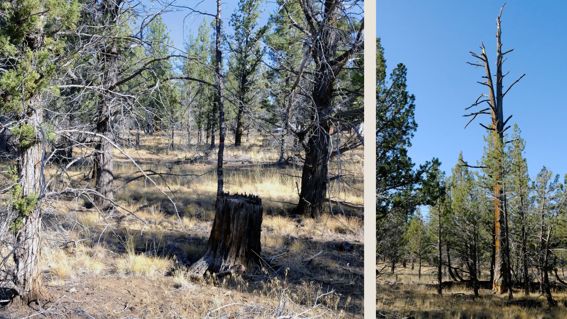
This results in ecosystems dominated by juniper. In sagebrush steppe, junipers grow to shade out the sage and eventually prevent anything else from growing by monopolizing all available soil moisture. In transitional zones junipers grow up under the ponderosa pines and pull moisture away, eventually stressing and the mature pine trees and leaving them susceptible to beetle attack.
I’ve noticed this dynamic on our property; lots of small junipers grow up around the pines. On the whole five acres there’s many young juniper and just one young ponderosa pine. Interestingly, there are stumps from the old-growth pines that used to cover the property, more pines than there are today. I’m guessing that the pines weren’t replaced because the the fast-growing juniper created a canopy that prevented the shade-intolerant ponderosa pines from seeding and growing up.
Where are the pines?
In light of the junipers’ aggressive colonization efforts, our general management strategy is to preserve the mature ponderosa pines and reduce the density of junipers.
As we plan for development of the property, it’s important to know where the pines are in order to work around them. This is often accomplished with a survey; a surveyor would be able to record the locations of trees over a certain diameter. However we don’t have a survey.
Another option would be to walk the property and record the coordinates of each tree. The only tool I have with GPS is my phone, which seems to have variable accuracy around 15-20 feet. That’s not accurate enough for me.
Working in QGIS, I decided to try to use freely available GIS datasets to identify the location of the ponderosa pine trees from aerial imagery.
Hand-classifying trees with satellite imagery
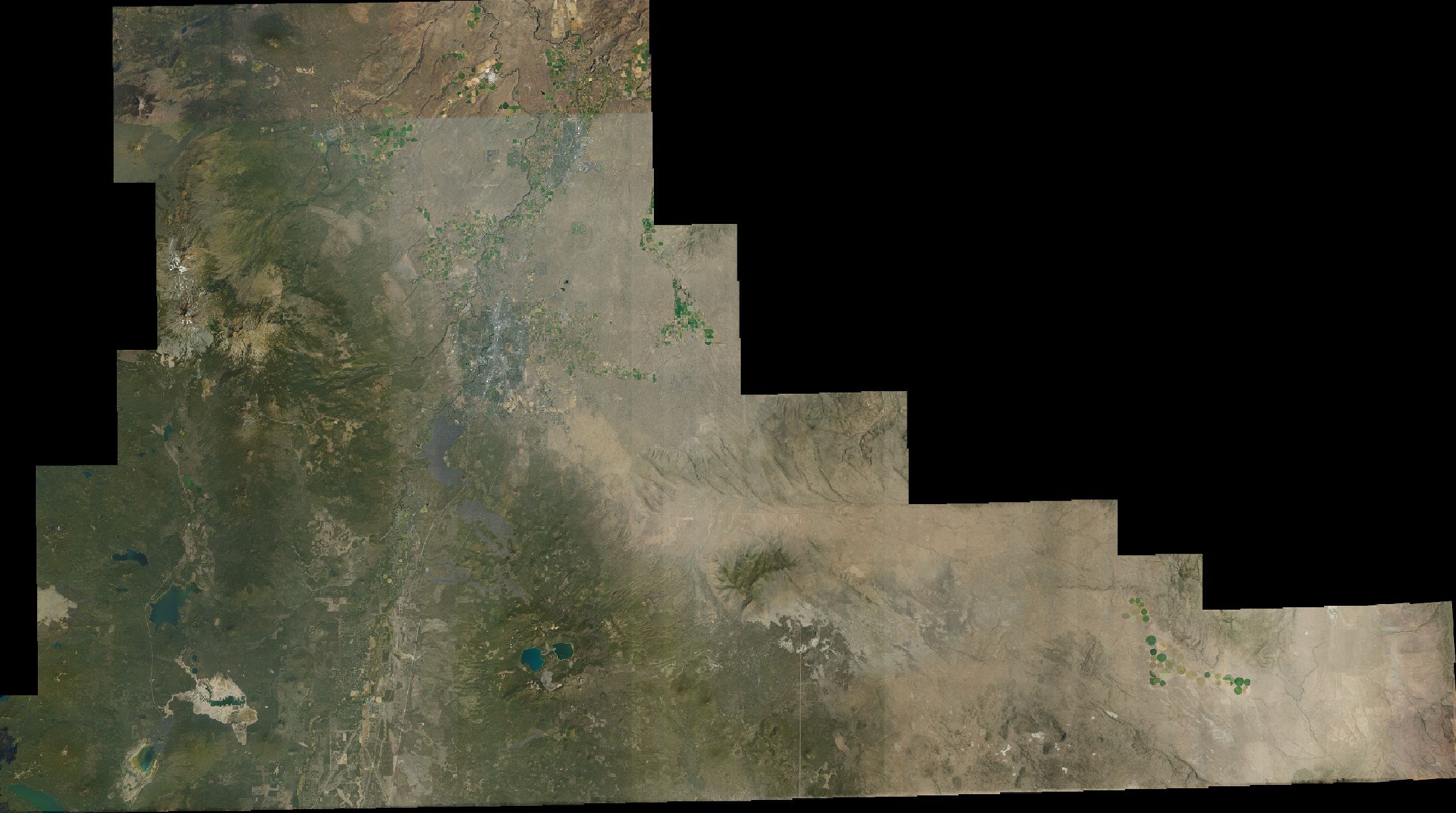
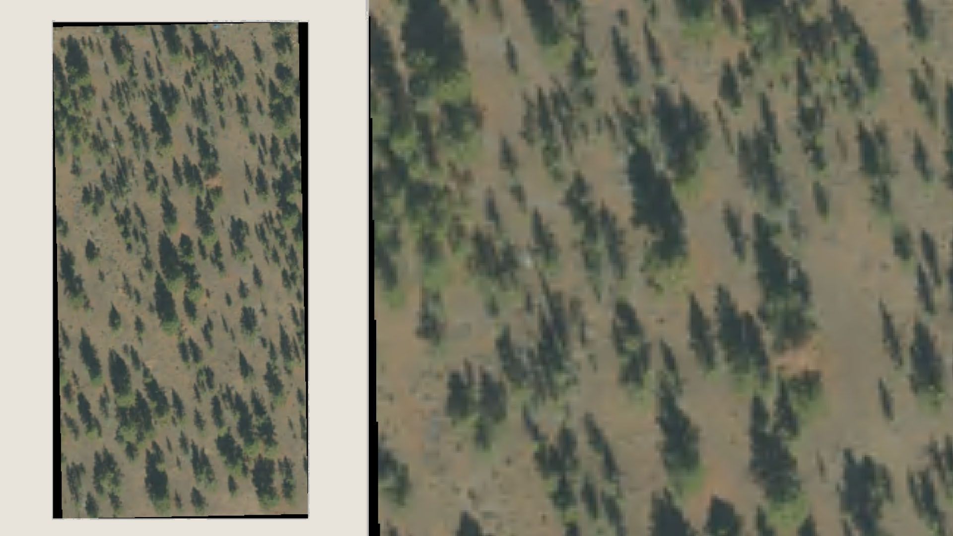
I started with satellite imagery available through the USDA’s National Agriculture Imagery Program. It isn’t limited to agricultural land; the dataset contains imagery for the entire CONUS in 60 or 30 centimeter per-pixel resolution.
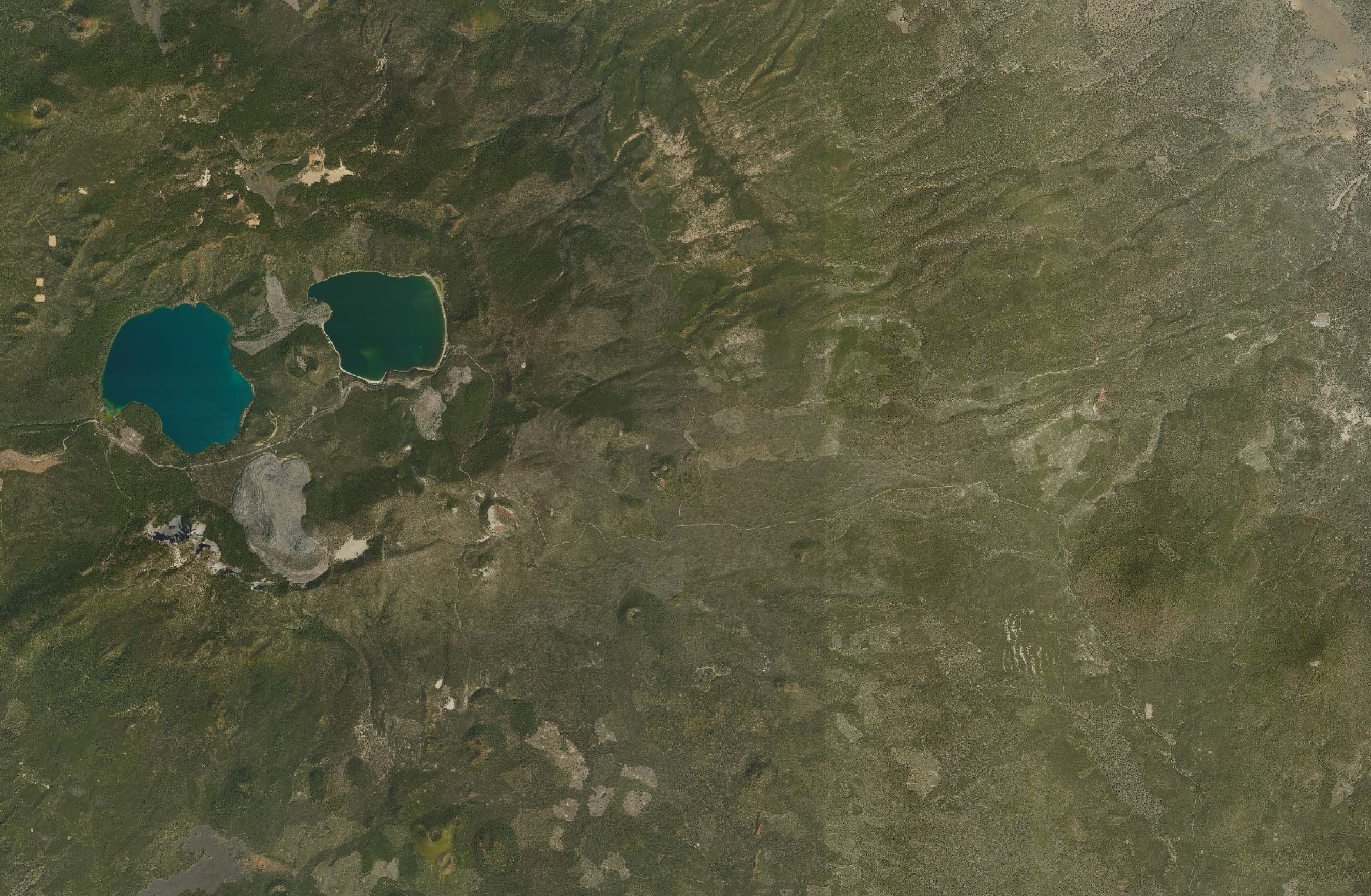
I began to pick out the locations of the ponderosa pines from the satellite images. I found myself relying on the length of the trees’ shadow to distinguish between the taller pines from the junipers. In areas where the shadows were unclear it wasn’t possible to positively identify specific tree locations. I’d need another method.
The shadows got me thinking about alternative data sources. Since the trees on the property are spaced out and don’t form a dense canopy, it could be possible to use aerially-captured Lidar data to detect them.
Algorithmically identifying trees with Lidar data
I don’t know if there’s a “proper” way to extract tree positions from Lidar data, but what follows is the path I took to arrive there while figuring it out as I went. It might not be optimal, but it ended up working.
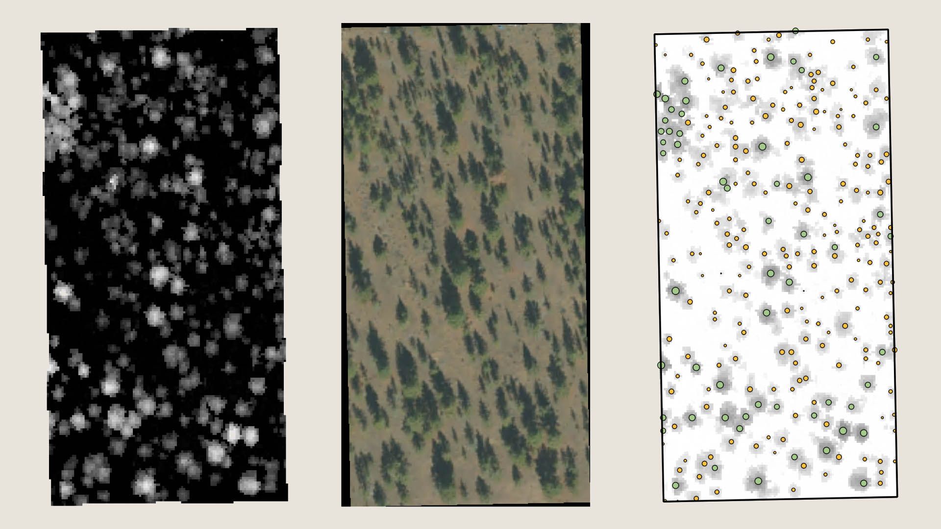
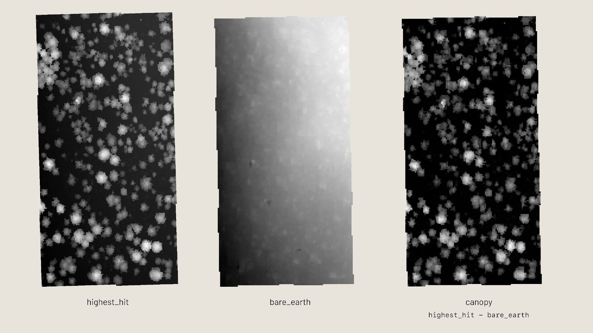
I found high-resolution Lidar data available through the State of Oregon’s Department of Geology and Mineral Industries. There’s two forms of Lidar that are useful here: highest hit and bare earth. Highest hit Lidar provides height readings for everything: each pixel represents the height of the underlying tree canopy, buildings, or ground. Bare earth is as it sounds: each pixel represents the height of the ground. Subtracting the two creates a canopy height map: the height of any trees or buildings off the ground.
The trees’ center points are the local maximum; the highest-value pixel in each cluster of non-zero value pixels. To find these highest-value pixels, I ran the GRASS GIS algorithm r.neighbors that creates a square around each pixel (5×5 in this case) and sets the pixel to the highest value in that square. I then subtracted the two rasters and set the locally highest-value pixels to 1.
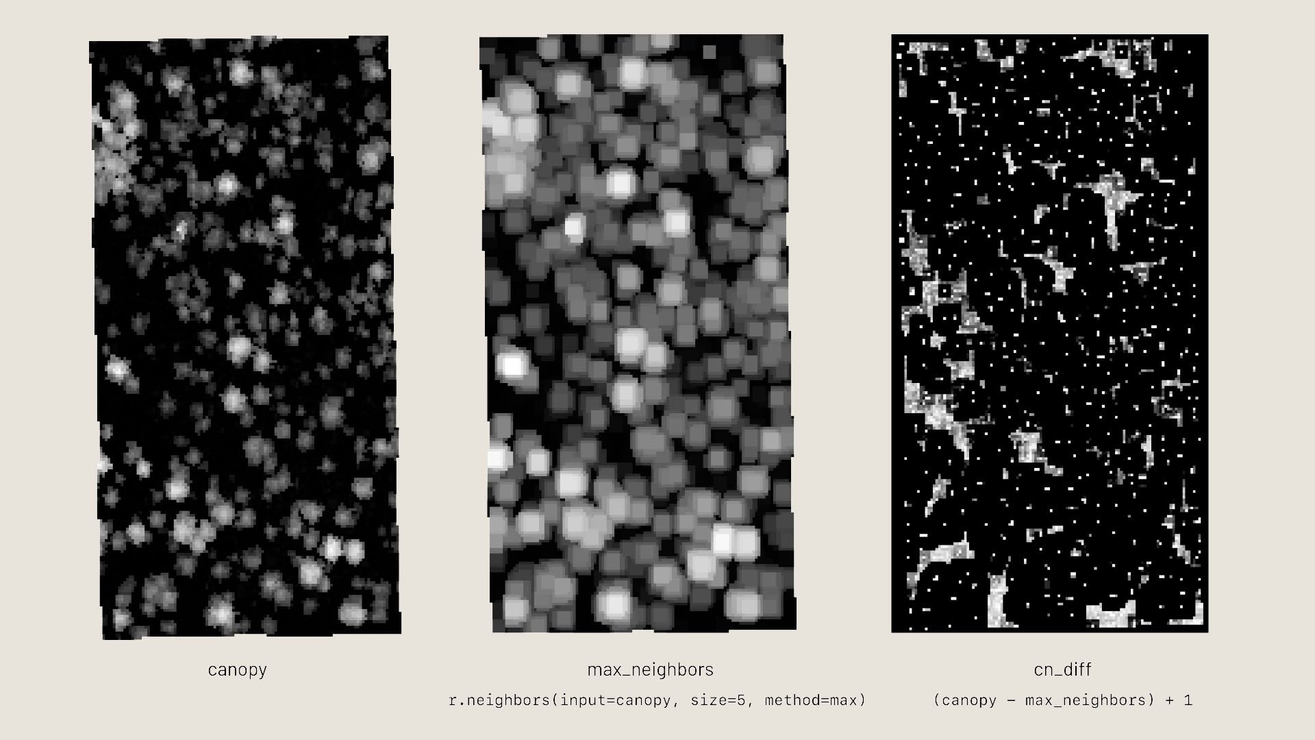
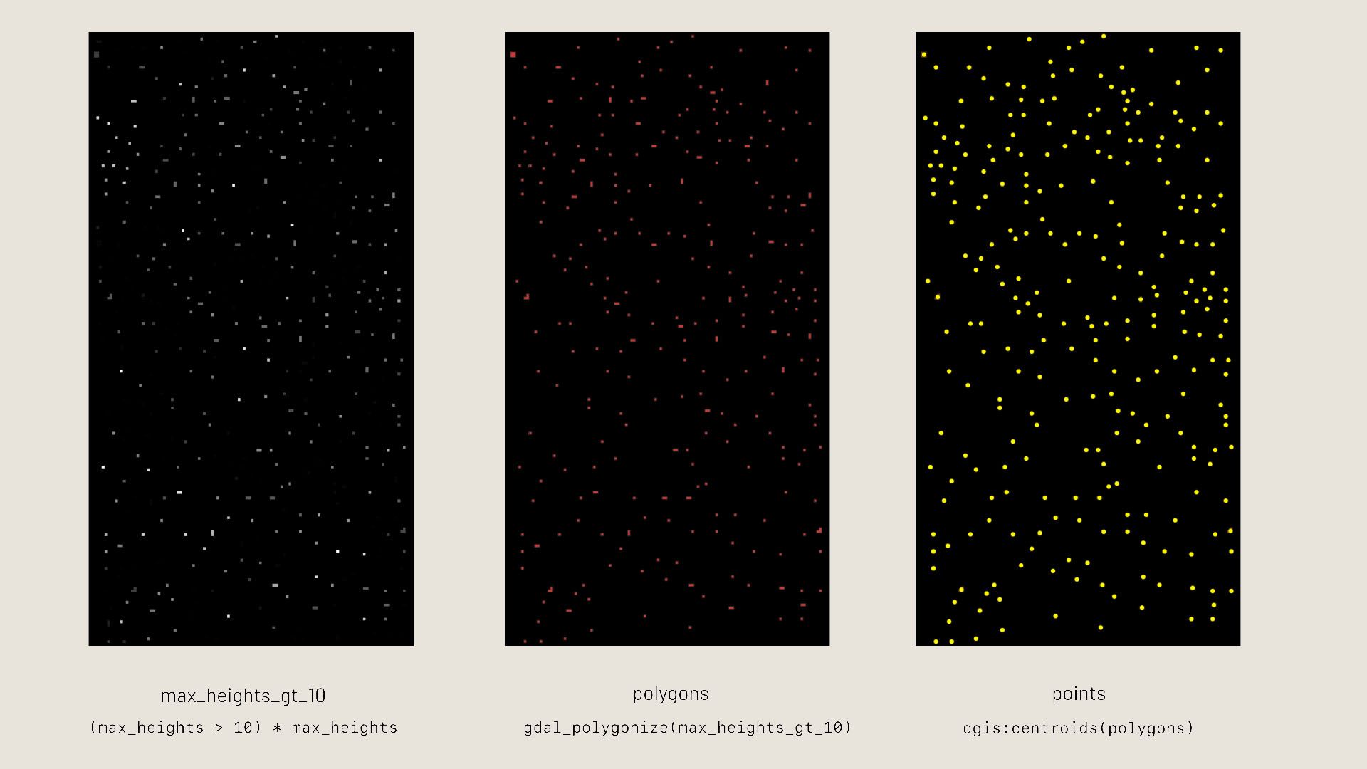
Next, I cleaned up the results by setting all non-one values to zero, creating a binary mask. However not all the points included in the mask are true local maximum. This is because when running the r.neighbors algorithm I set the square size to 5, so in regions larger than 5 pixels that weren’t part of a tree the background noise was amplified and a very small maximum was found. To clean this noise up, I multiplied the mask with the canopy map to get the height values for each maximum, then filtered out any points with values less than 10.
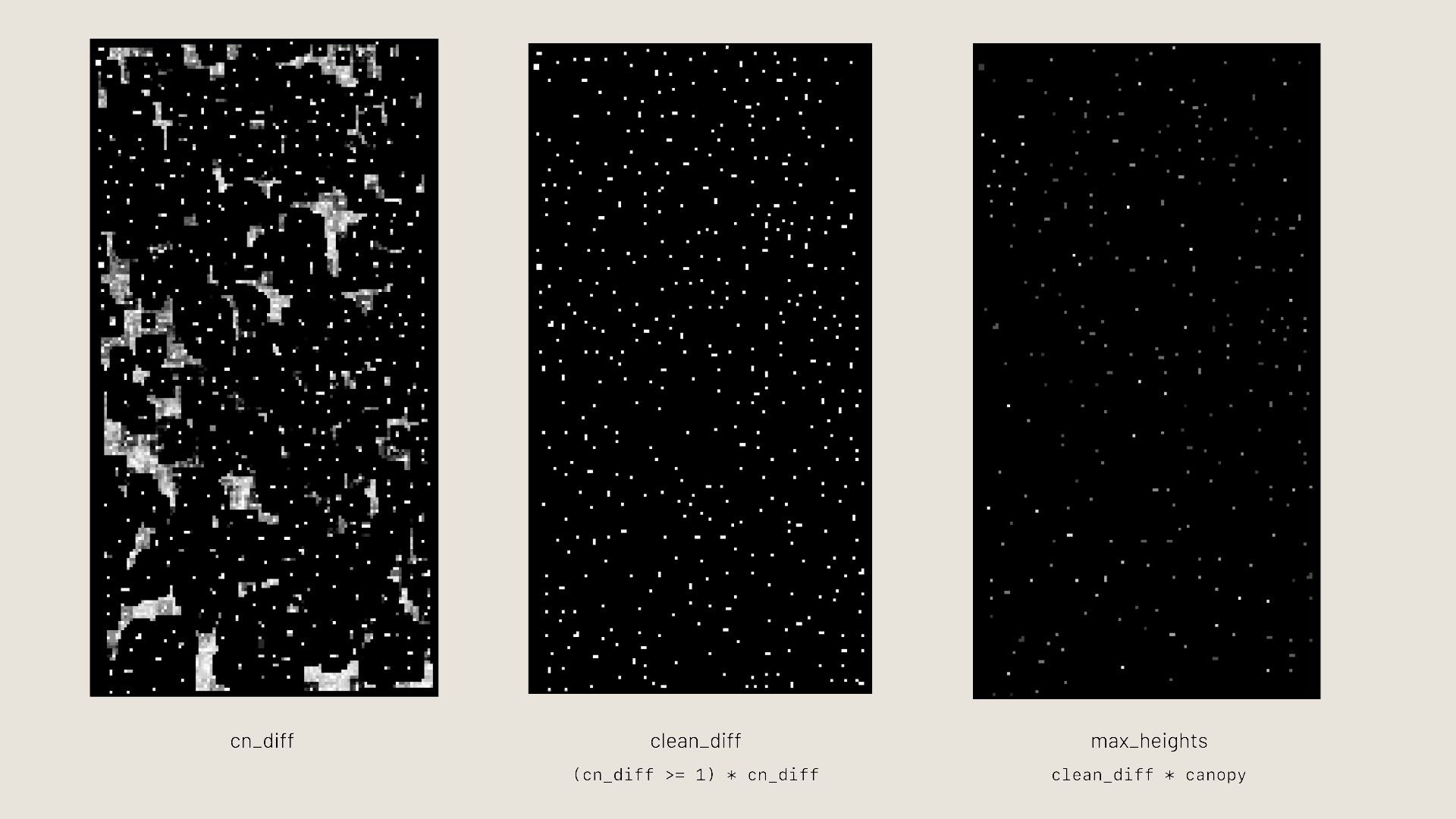
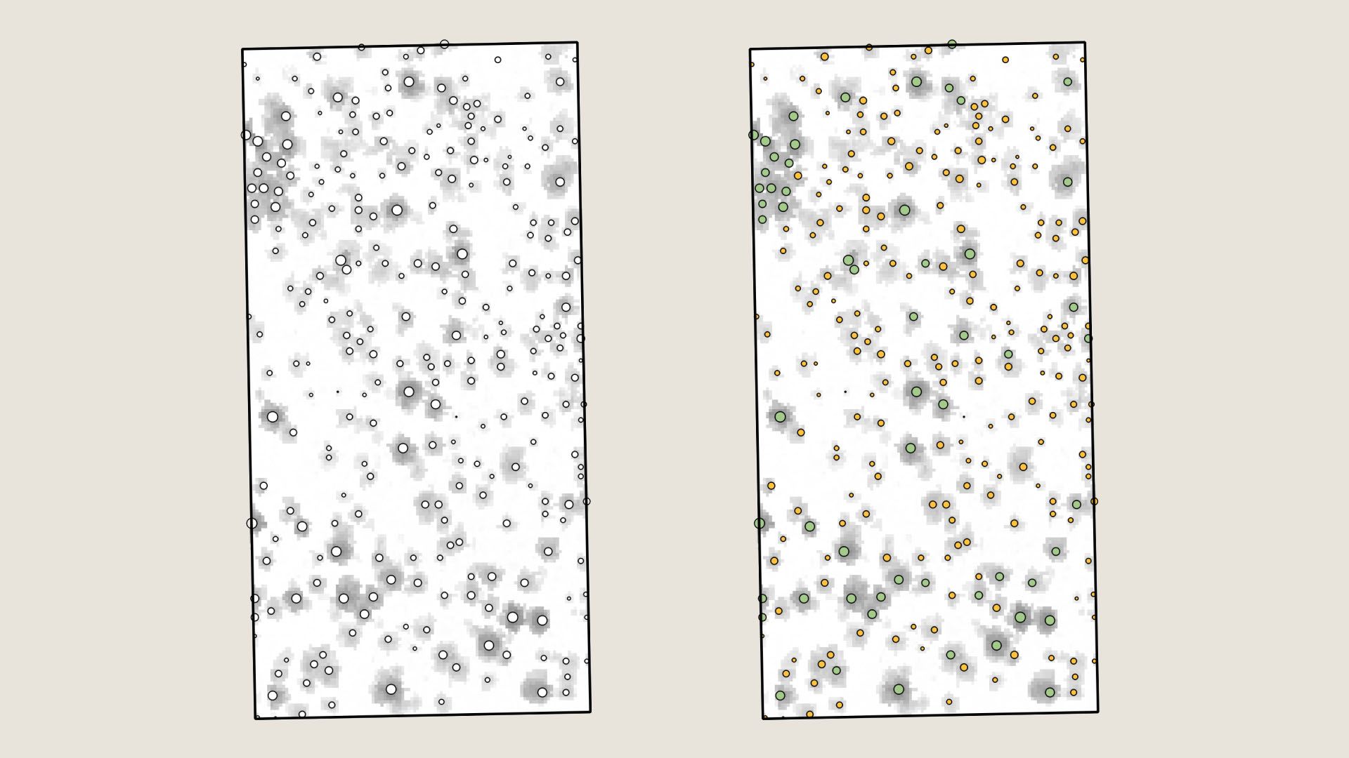
To create points representing the tree positions I converted the pixels to polygons with gdal_polygonize, then ran the QGIS centroid algorithm to find the centroids of each single-pixel sized polygon.
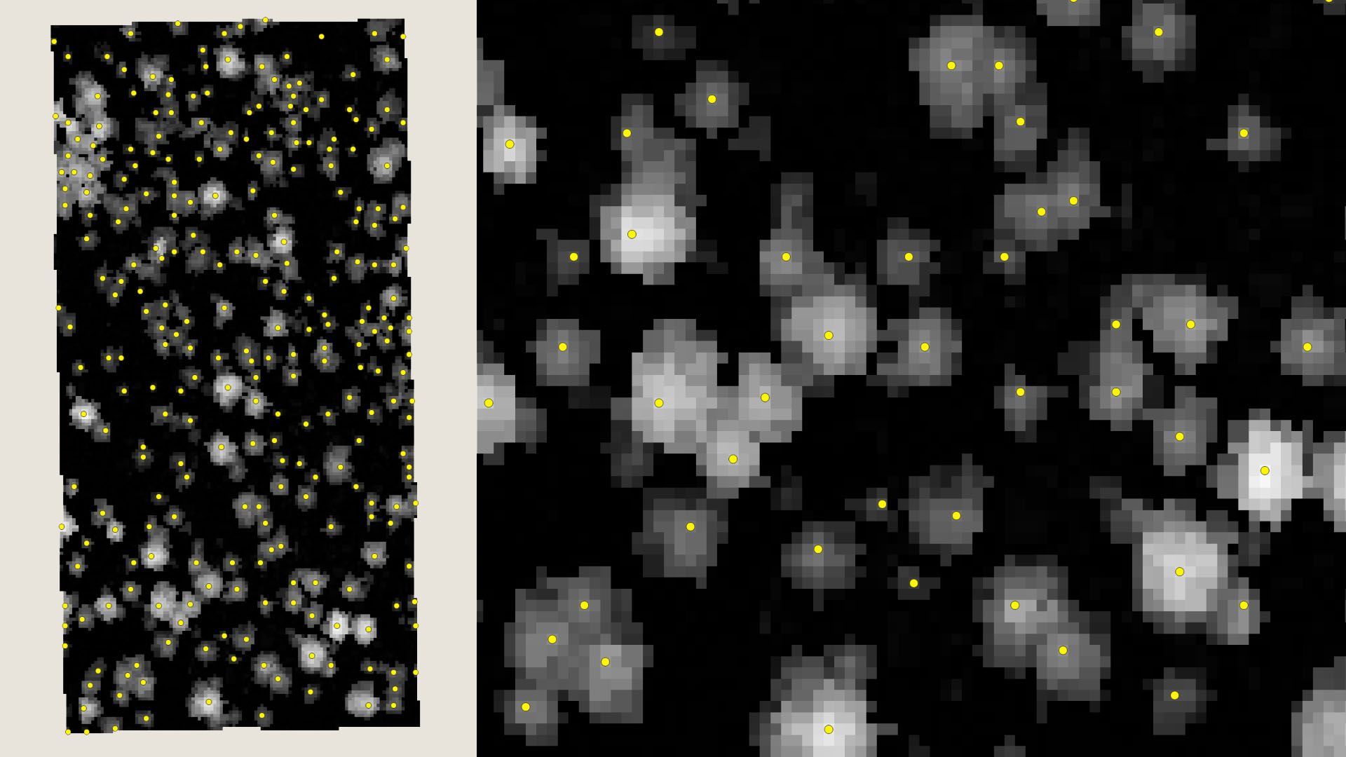
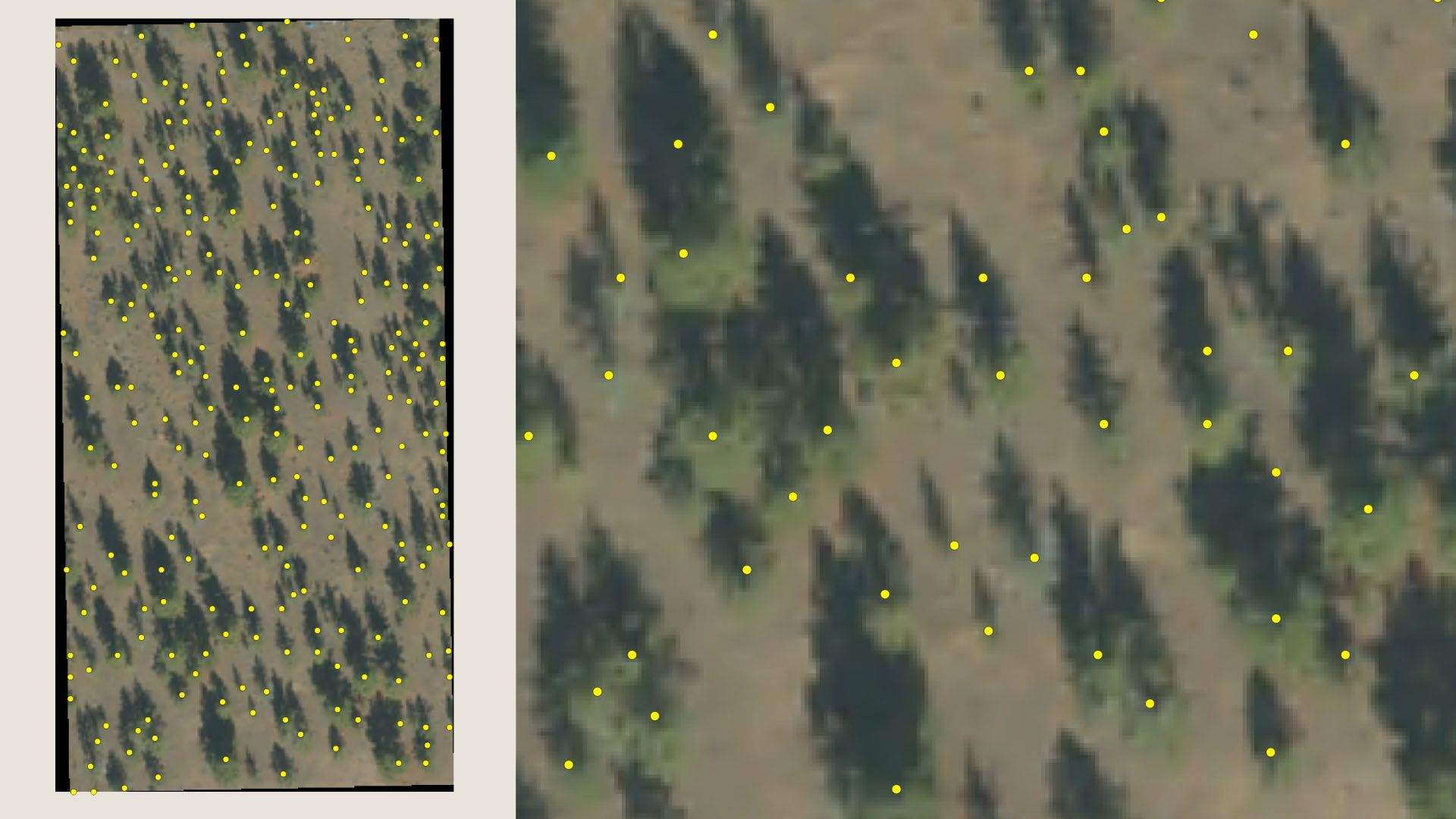
The results are decent! At most the points appear to be off a few pixels. With each pixel being 30cm, the accuracy is conservatively around 90cm, though most points appear dead on.
With each tree associated with its height from the canopy map, I made a histogram of all the tree heights. There are 275 trees on the property, most falling in the 20-40ft height range.
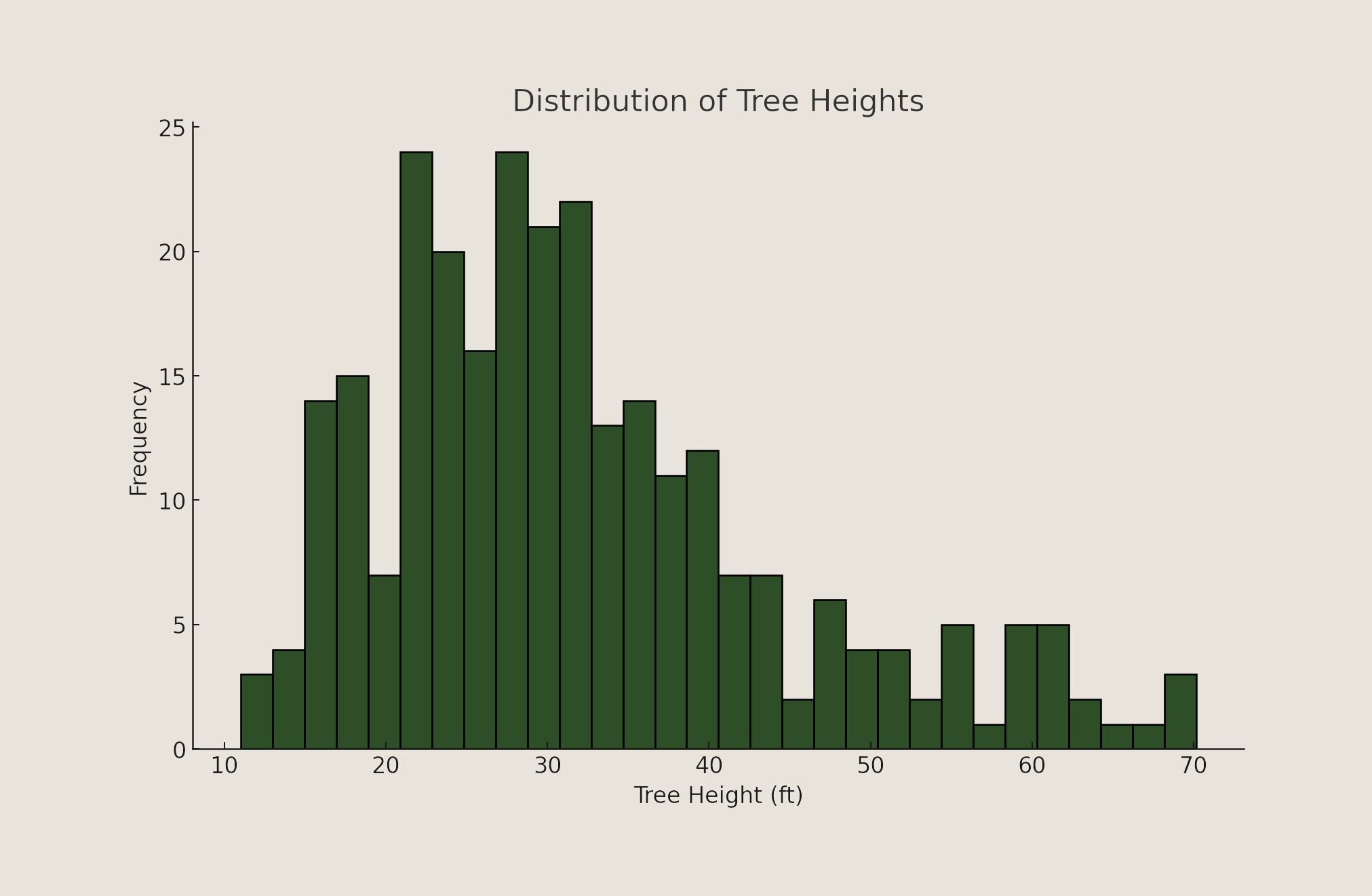
The ponderosa pines are more mature and taller than the junipers, starting around 40ft and up. Using this rough heuristic it’s easy to estimate which trees are pines.
Next up: verification and thinning trees
The next step is to take this survey and walk the site to verify the trees detected through this process are really there and marked as the correct species. After that I’ll mark junipers that should be removed around the pines and in areas where they’re growing too densely. Then I’ll get out a chainsaw and implement the plan.
⁂