Creating high-resolution raster terrain tiles from LIDAR source DEMs

In this post, I develop a method for generating terrain tiles for use in digital interactive maps. I integrate USGS digital elevation models with the highest-resolution available LIDAR data in a mosaic, then create TerrainRGB tiles.

At the foundation of every good topographic map is some representation of the terrain. Whether the goal is to build a rich three dimensional Google Earth-like map or a two dimensional topographic hiking map with elevation contours, we’ll need a way to indicate elevation.

By the end of this post, we’ll have created high-resolution terrain tiles that can be viewed in the browser, to create three dimensional experiences like this:

Drag to rotate

This post documents the method I used to create these elevation tiles. I’m not a GIS expert; this is just a method that I figured out with the internet and several weeks of experimentation. Maybe there’s a better, more efficient way to go about it. If so let me know.

I’ll use only open source tools, including GDAL, rasterio, pmtiles, and MapLibre GL JS. The datasets are freely accessible from U.S. federal and state agencies (you’ve paid for them with your taxes; better to make your own tiles than pay Google for theirs!) I haven’t looked into data sources for regions outside the U.S. but the process should be the same.

I should also note that this method is working well for smaller regions, but I haven’t tried it for larger areas like an entire state. The primary bottleneck to building terrain tiles for larger regions is the amount of RAM and CPU cores you’d need to process the tiles in a reasonable amount of time. I generated all the tiles for this post on my M2 MacBook Pro with 16GB of RAM. A future post will document the process of generating terrain tiles for larger areas.

Table of Contents

• USGS digital elevation models
  • Downloading DEMs
  • Projections
• Cutting DEMs into TerrainRGB tiles
  • Deriving maximum zoom level from DEM resolution
  • Generating tiles
• Incorporating high-resolution LIDAR data
  • Reprojecting and mosaicing LIDAR DEMs
  • Choosing a resolution to limit file size
  • Upsampling lower-quality DEMs
• Visualizing the terrain
  • Contours
  • Elevation profile
• Next: larger regions

USGS digital elevation models

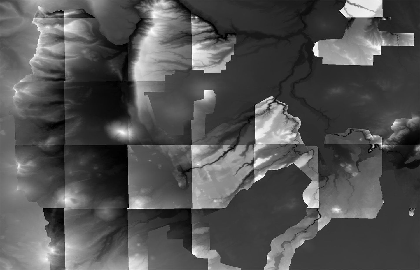
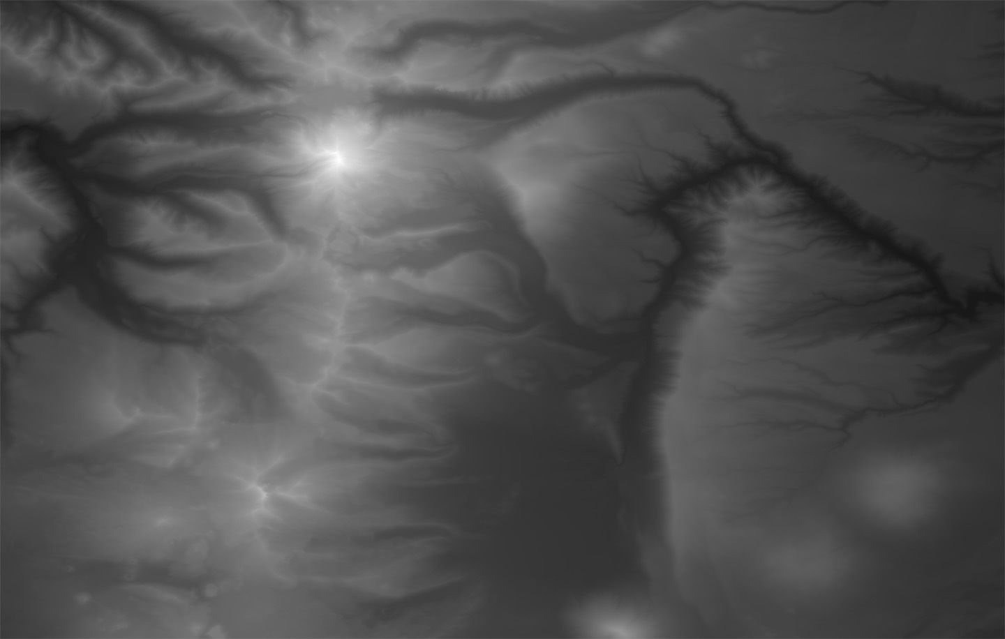
Raw elevation data comes in the form of digital elevation models (DEMs): raster images that represent the elevation of a region. Each pixel’s value represents an elevation.

USGS provides DEMs for the United States in several resolutions. The highest-resolution option that covers the entire U.S. is the ⅓ arc-second dataset. It’s available for free without restriction.

Downloading DEMs

We can download DEMs from the National Map—a service provided by USGS to download public GIS data—via its API. I wrote a small CLI to download DEMs for a given bounding box.

It can be used like this:

python download_elevation_data.py \
    --bbox="-122.011414,46.655136,-121.467590,47.026401" \
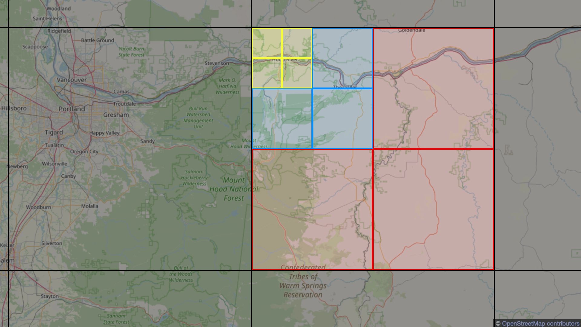
    --dataset="National Elevation Dataset (NED) 1/3 arc-second"

DEMs are provided at fixed sizes, so a bounding box might include multiple:

data/
    sources/
        USGS_13_n47w122_20180208.tif
        USGS_13_n47w123_20220505.tif
        USGS_13_n48w123_20200107.tif
        USGS_13_n47w122_20211129.tif
        USGS_13_n47w123_20230608.tif
        ...

Projections

These DEMs are projected in WGS84, which can serve as both a horizontal and vertical datum. In this case it’s just used horizontally, meaning that the x/y coordinates of the image correspond to latitude and longitude. The z component—in this case the elevation—is in the vertical datum NAVD88. NAV88 is based on a network of known physical leveling points spread across North America all tied to a tidal benchmark in Quebec (you can find the locations of these control points in a map provided by the National Geodetic Survey). NAVD88 is meant to represent elevation above sea level. It may be reported in meters or feet.

Cutting DEMs into TerrainRGB tiles

The next step is tiling the DEMs. Tiling means cutting the large raster images into many smaller images at different resolutions. These tiles allow rendering software to load a small piece of the image without loading the entire thing. Tiles are cut at distinct zoom levels, where each zoom level is twice as large as the previous. Zoom levels usually range from 0 (one tile of the entire earth) to 20 (1+ trillion tiles representing areas of mid-sized buildings).

Because there are multiple representations of the image at different zoom levels, tiled images can be very large. Files grow exponentially as each additional zoom level increases the file size by a factor of 4.

Deriving maximum zoom level from DEM resolution

To prevent generating tiles for the DEMs beyond their full resolution, we need a method to find the maximum zoom level that can be supported by a given raster.

The challenge is to relate pixel size—which can be found easily with GDAL—to zoom level.

We can start with a formula from the OpenStreetMap wiki used to determine the size of a tile at a latitude $\phi$ and zoom level $z$:

$$S_{tile\ (m)} = \frac{C \times \cos \phi}{2^{z}}$$

Here $C$ is the equatorial circumference of the Earth in meters. Note that $C$ is not actually the circumference of earth, it’s an estimate based on the WGS84 reference ellipsoid of $40,075,016.686m$.

This gives us the size of a tile in meters. The tiles we’re generating are 512px wide and tall, so the pixel size is:

$$S_{pixel\ (m)} = \frac{S_{tile\ (m)}}{512}$$

This is enough information to rearrange the formulas to solve for $z$, given a known pixel size:

$$z = \log_2\bigg(\frac{C \times \cos \phi}{512 \times S_{pixel\ (m)}}\bigg)$$

Now we can find $z$ for our rasters. To find the pixel size of the DEMs, I ran gdalinfo on one:

gdalinfo data/sources/USGS_13_n45w122_20140718.tif

This prints out a variety of metadata, including:

Pixel Size = (0.000092592164936,-0.000092592164936)

Since the image is in WGS84, the unit the pixel is reported in is degrees latitude and longitude. We’ll need to convert the pixel size to meters to work with our formula.

We start with a formula from Wikipedia to approximate the meters per one degree latitude in WGS84:

$$\Delta^{1\degree}_{latitude} = 111,132.954 - 559.822 \times \cos 2 \phi + 1.175 \times \cos 4 \phi$$

This gives a distance accurate to $0.01m$ for $\phi \pm 0.5$.

The idea is to select the latitude $\phi$ at the center of the raster and use it to find $\Delta^{1\degree}_{latitude}$.

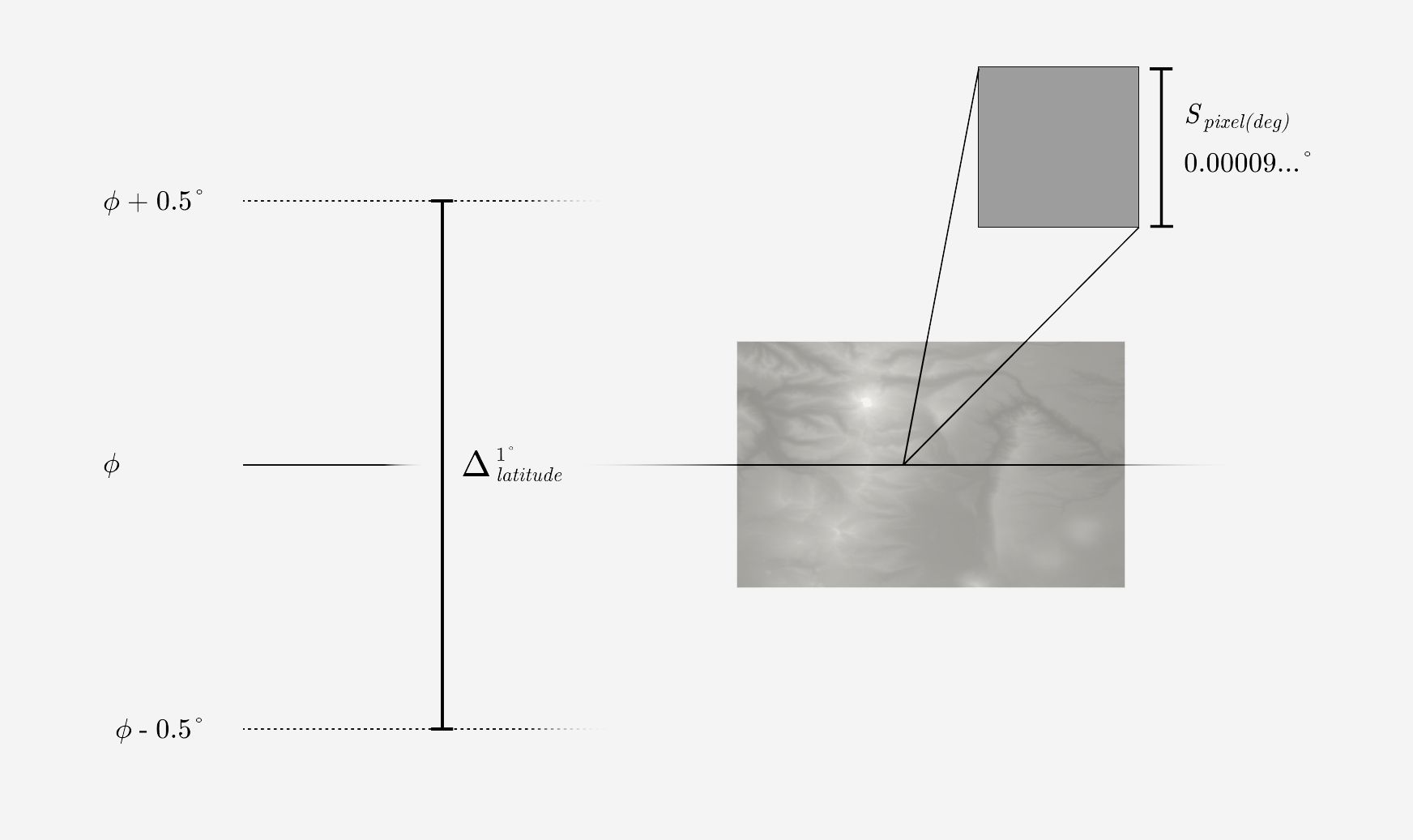
Since the pixel height value is a fraction of one degree latitude, we can multiply it by $\Delta^{1\degree}_{latitude}$ to get the pixel size in meters.

$$S_{pixel\ (m)} = S_{pixel\ (deg)} \times \Delta^{1\degree}_{latitude}$$

For $\phi = 44.5\degree$, one degree of latitude is approximately $111,113m$. So our pixel size is approximately $10.288m$.

This means that the maximum zoom level we can support is 12.41; tiles after this zoom level won’t contain any new information.

Here’s a python implementation of the full process:

import math

C = 40075016.686

def get_max_zoom(latitude, pixel_size_degrees):
    meters_per_degree = 111123.954 - 559.822 * math.cos(math.radians(2 * latitude)) + 1.175 * math.cos(math.radians(4 * latitude))
    pixel_size_meters = pixel_size_degrees * meters_per_degree
    max_z = math.log2((C * math.cos(math.radians(latitude))) / (512 * pixel_size_meters))
    return max_z

Generating tiles

We’ll need to convert the DEMs to an image format that’s easily readable by a browser; the 10812x10812px grayscale geotiff images provided by USGS are difficult to work with outside of GIS software. Mapbox created a format called TerrainRGB that’s designed to represent elevation data as RGB images that can be PNGs or WEBPs.

The elevation can be decoded from a pixel value with this equation:

$$elevation = -10000 + ((R \times 256 \times 256 + G \times 256 + B) \times 0.1)$$

Once the images are converted to TerrainRGB, we’ll tile them so they can be viewed in the browser.

To begin, we build a dataset that combines all the DEMs virtually as a VRT. This will allow us to operate on all the DEMs without needing to combine them into a single image. Using GDAL’s gdalbuildvrt:

gdalbuildvrt \
    -overwrite \
    -srcnodata -9999 \
    -vrtnodata -9999 \
    data/temp/dem.vrt \
    data/sources/*.tif

Next we’ll convert to TerrainRGB images and tile in one step. For this we’re using the python package rasterio with an extension from Mapbox called rio-rgbify. Previously we found the maximum zoom we can generate with this dataset is 12.41, so I rounded up and set --max-z 13.

rio rgbify \
    --base-val -10000 \
    --interval 0.1 \
    --min-z 1 \
    --max-z 13 \
    --workers 10 \
    --format webp \
    data/temp/dem.vrt \
    data/output/elevation.mbtiles

Note that rio-rgbify is an abandoned project and has at least one bug that you’ll need to manually fix to get this to work.

Once run, rio-rgbify produces a mbtiles file, a format created by Mapbox to store pyramidal tiles. However it’s missing a metadata field denoting the boundaries of the dataset, so I wrote a script to add those:

python add_metadata.py \
    --input-file="data/output/elevation.mbtiles"

I prefer to work with PMTiles, so we’ll convert from mbtiles with the pmtiles CLI:

pmtiles convert \
    data/output/elevation.mbtiles \
    data/output/elevation.pmtiles

Here’s what the tiles look like:

Drag to pan, double click to zoom

This single USGS DEM tile resulted in a 96MB pmtiles archive containing zoom levels 1-13.

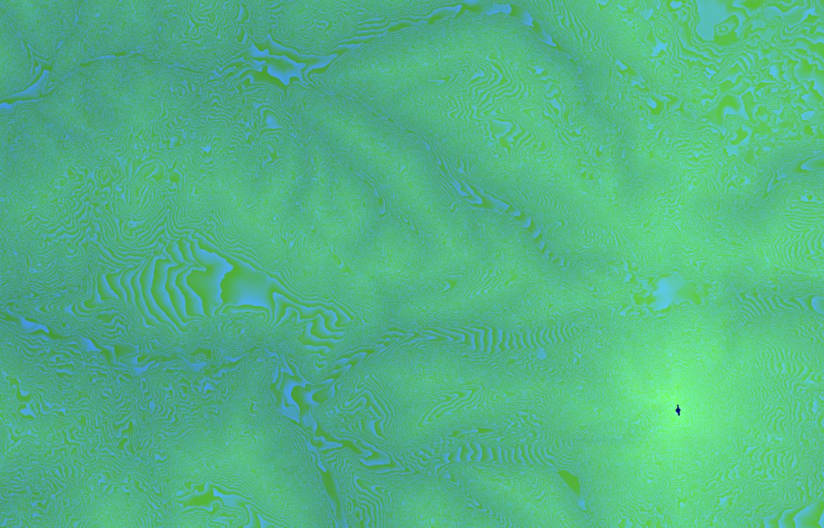
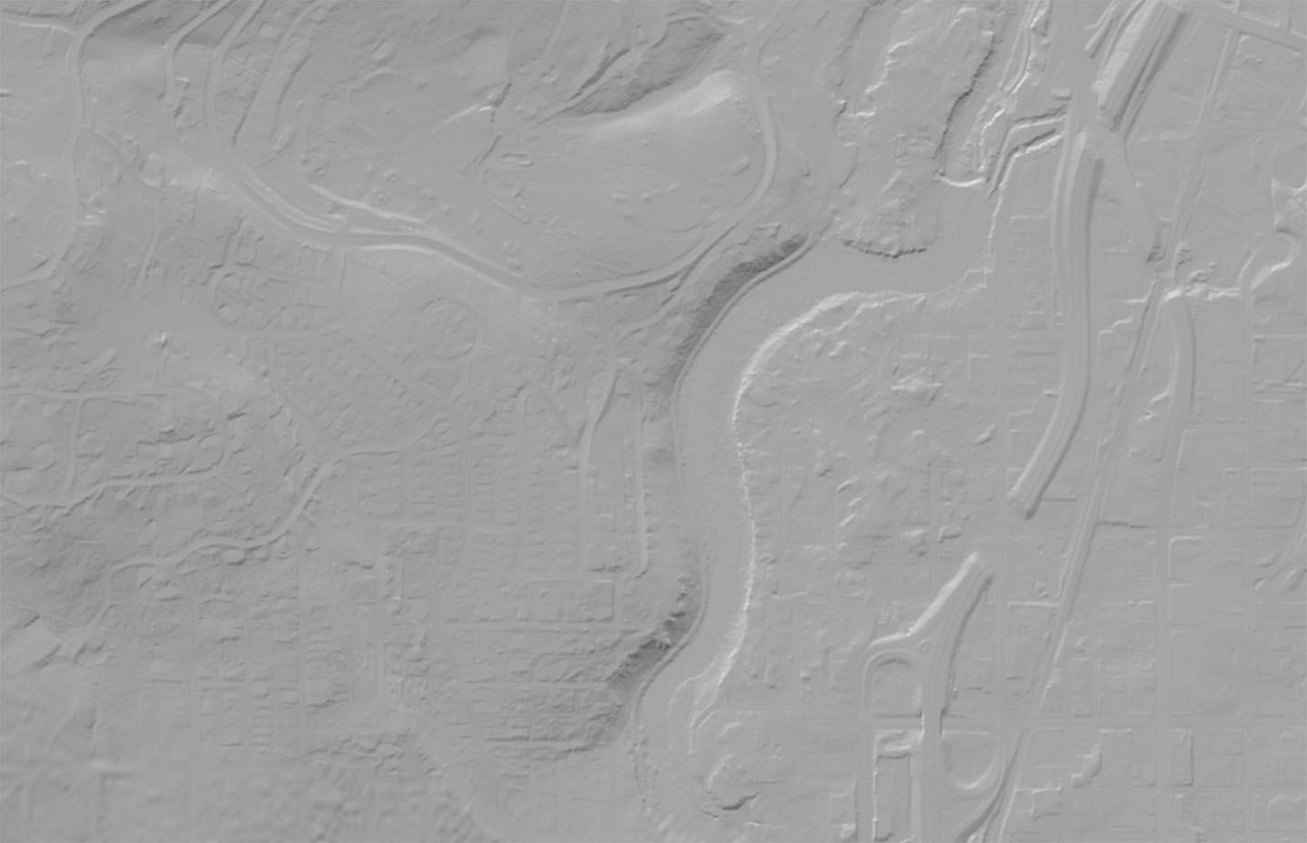
TerrainRGB tiles aren’t meant to be shown as-is; they should be decoded before visualizing. They can be styled as a hillshade—a three dimensional representation of the terrain using a artificial light source—in MapLibre GL JS. The style spec for hillshading looks like this:

{
  "id": "hillshade",
  "type": "hillshade",
  "source": "elevation",
  "source-layer": "elevation",
  "paint": {
    "hillshade-exaggeration": 0.8,
    "hillshade-shadow-color": "#5a5a5a",
    "hillshade-highlight-color": "#ffffff",
    "hillshade-accent-color": "#5a5a5a",
    "hillshade-illumination-direction": 335,
    "hillshade-illumination-anchor": "viewport"
  }
}

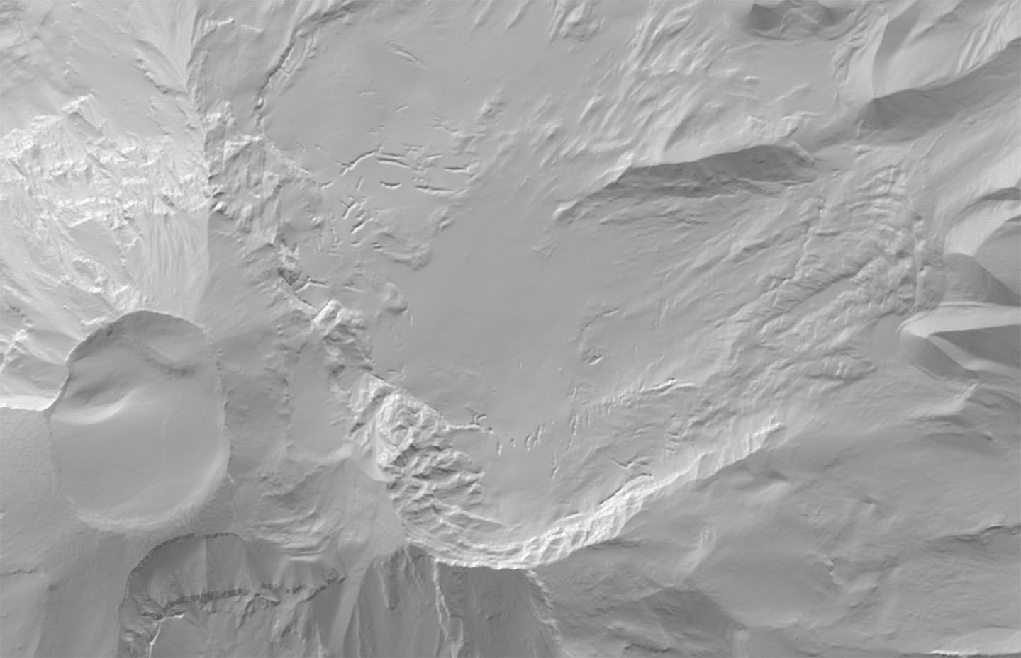
Here’s the result:

Drag to pan, double click to zoom

This could make a decent base layer. However, there are some areas around dramatic features that could use some more work. The spires of Smith Rock, for example, become blobby due to the relatively low-resolution DEM source data.

Incorporating high-resolution LIDAR data

For the highest-resolution elevation dataset, the answer is usually LIDAR. It’s trickier to find LIDAR data for an area of interest since there’s no centralized location where all LIDAR data is stored (in the United States, at least). Here are some repositories that had data for areas I’m interested in:

• U.S. Interagency Elevation Inventory (best)
• USGS 3DEP LIDARExplorer
• NOAA Digital Coast
• Oregon Department of Geology and Mineral Industries LIDAR Viewer
• Washington State Department of Natural Resources LIDAR Portal

Another complication is that LIDAR data is usually grouped into distinct project areas where it’s been collected. As far as I know there’s no way to download all data for an arbitrary bounding box.

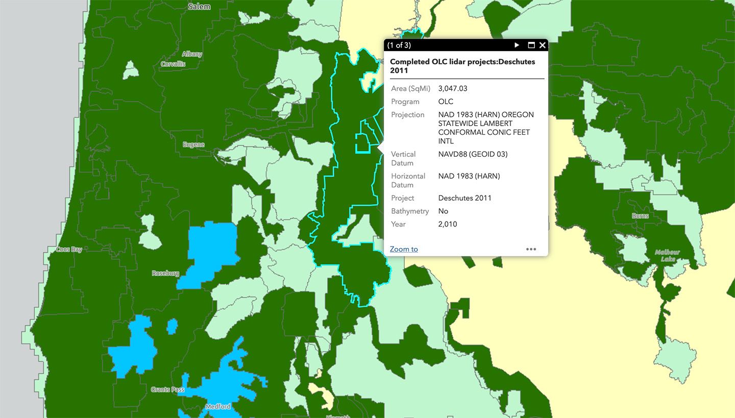
I decided to focus on an area within a larger LIDAR acquisition project. Since each project is composed of multiple LIDAR-derived DEMs, I checked each to determine if it intersected my region of interest and discarded everything that didn’t. This was an inefficient approach but it worked for this small region.

With the LIDAR DEMs downloaded, we can check their resolution and projection:

gdalinfo data/sources/be_44120d8b.tif

The relevant parts:

Coordinate System is:
    COMPOUNDCRS["NAD83(HARN) / Oregon GIC Lambert (ft) + NAVD88 height (ft)",
...
Pixel Size = (3.000000000000000,-3.000000000000000)
...
NoData Value=-3.4028235e+38

The DEMs are projected in Oregon GIC Lambert, so the pixel size unit is feet. Approximately $1m$ per pixel is much higher resolution than the $10.288m$ per pixel standard ⅓ arc-second DEMs.

In order to tile the rasters, we’ll need to set a consistent resolution, projection, and no-data value between the LIDAR DEMs and the standard DEMs.

Reprojecting and mosaicing LIDAR DEMs

To reproject the rasters, we’ll use gdalwarp. The details of this step will depend the project, as there are many possible projections the LIDAR rasters could be delivered in. In this case, it was Oregon GIC Lambert (EPSG:2992).

As before, we’ll start by building a VRT of all the LIDAR input files and set a new no-data value:

gdalbuildvrt \
    -overwrite \
    -vrtnodata -9999.0 \
    data/temp/lidar.vrt \
    data/sources/be*.tif

I had difficultly reprojecting the rasters to WGS84 in a single step since the LIDAR rasters have different horizontal datums but the same vertical datum (with the exception of the units). So I ended up splitting it out into two separate steps. In the first, we reproject on the horizontal datum only (with -novshift) from Oregon GIC Lambert (EPSG:2992) to WGS84 (EPSG:4326). We’re also trimming the result (with -te) to exactly fit the bounding box since some LIDAR rasters might exceed the bounds.

gdalwarp \
    -overwrite \
    -s_srs EPSG:2992 \
    -t_srs EPSG:4326 \
    -dstnodata -9999.0 \
    -novshift \
    -r near \
    -te -122.0005536 43.9994457 -120.9994471 45.0005522 \
    -of GTiff \
    -multi \
    -wo NUM_THREADS=10 \
    data/temp/lidar.vrt \
    data/temp/lidar.tif

Both the LIDAR rasters and standard rasters use NAVD88 for the vertical datum, but the LIDAR rasters are in feet while the standard ones are in meters. We’ll convert to meters with gdal_calc for consistency:

gdal_calc \
    -A data/temp/lidar.tif \
    --outfile=data/temp/lidar.tif \
    --calc="A*0.3048"

Choosing a resolution to limit file size

As before, we can calculate the maximum zoom level that can be supported by the LIDAR raster’s resolution. The LIDAR pixel size:

gdalinfo data/temp/lidar.tif

Pixel Size = (0.000009817175778,-0.000009817175778)

Using our formula from before:

get_max_zoom(44.5, 0.000009817175778)

We get a maxiumum $z$ of 15.64, so we’ll round up to 16.

To get a sense for how much this would increase the file size, the previous version stopped at zoom level 13. There were 816 tiles at this level with an average size of 100KB each. Extrapolating:

• Zoom 14: $816 \times 4 = 3,264$ tiles, 326.4MB at this zoom level
• Zoom 15: $3,264 \times 4 = 13,056$ tiles, 1.3GB at this zoom level
• Zoom 16: $13,056 \times 4 = 52,224$ tiles, 5.2GB at this zoom level

This would produce a file with a maximum size of 6.9GB. Note that this is an upper bound since the bounding box I’m using is rectangular and many of the tiles on the edges will be blank. We’ll generate up to zoom level 15 for now to keep the file smaller.

To speed up computation, we can lower the resolution of the LIDAR rasters. We need to find the target resolution to set to support up to zoom level 15.

We can rearrange the formulas from before to get the pixel size in meters for a zoom level $z$:

$$S_{pixel\ (m)} = \frac{C}{2^z \times 512}$$

Then convert it back to degrees at a latitude $\phi$:

$$S_{pixel\ (deg)} = \frac{S_{pixel\ (m)}}{111,132.954 - 559.822 \times \cos 2 \phi + 1.175 \times \cos 4 \phi}$$

Here’s a python implementation:

import math

C = 40075016.686

def get_pixel_size_at_zoom(latitude, zoom):
    meters_per_degree = 111123.954 - 559.822 * math.cos(math.radians(2 * latitude)) + 1.175 * math.cos(math.radians(4 * latitude))
    pixel_size_meters = C / (math.pow(2, zoom) * 512)
    pixel_size_degrees = pixel_size_meters / meters_per_degree
    return pixel_size_meters, pixel_size_degrees

So at latitude $44.5\degree$ and a maxiumum zoom level 15 the pixel size we should use is $0.000021497547$ degrees per pixel.

Now when we create a VRT combining the LIDAR DEMs and standard DEMs, we can explicitly set this resolution:

gdalbuildvrt \
    -overwrite \
    -vrtnodata -9999.0 \
    -resolution user \
    -tr 0.000021497547 -0.000021497547  \
    data/temp/dem.vrt \
    data/sources/USGS*.tif \
    data/temp/lidar.tif

Upsampling lower-quality DEMs

While this new resolution is lower than the LIDAR rasters’ original resolution, it’s larger than the standard DEMs’ resolution. Because we’re upsampling the standard DEM, we’ll need to specify a resampling method so the image doesn’t appear pixelated.

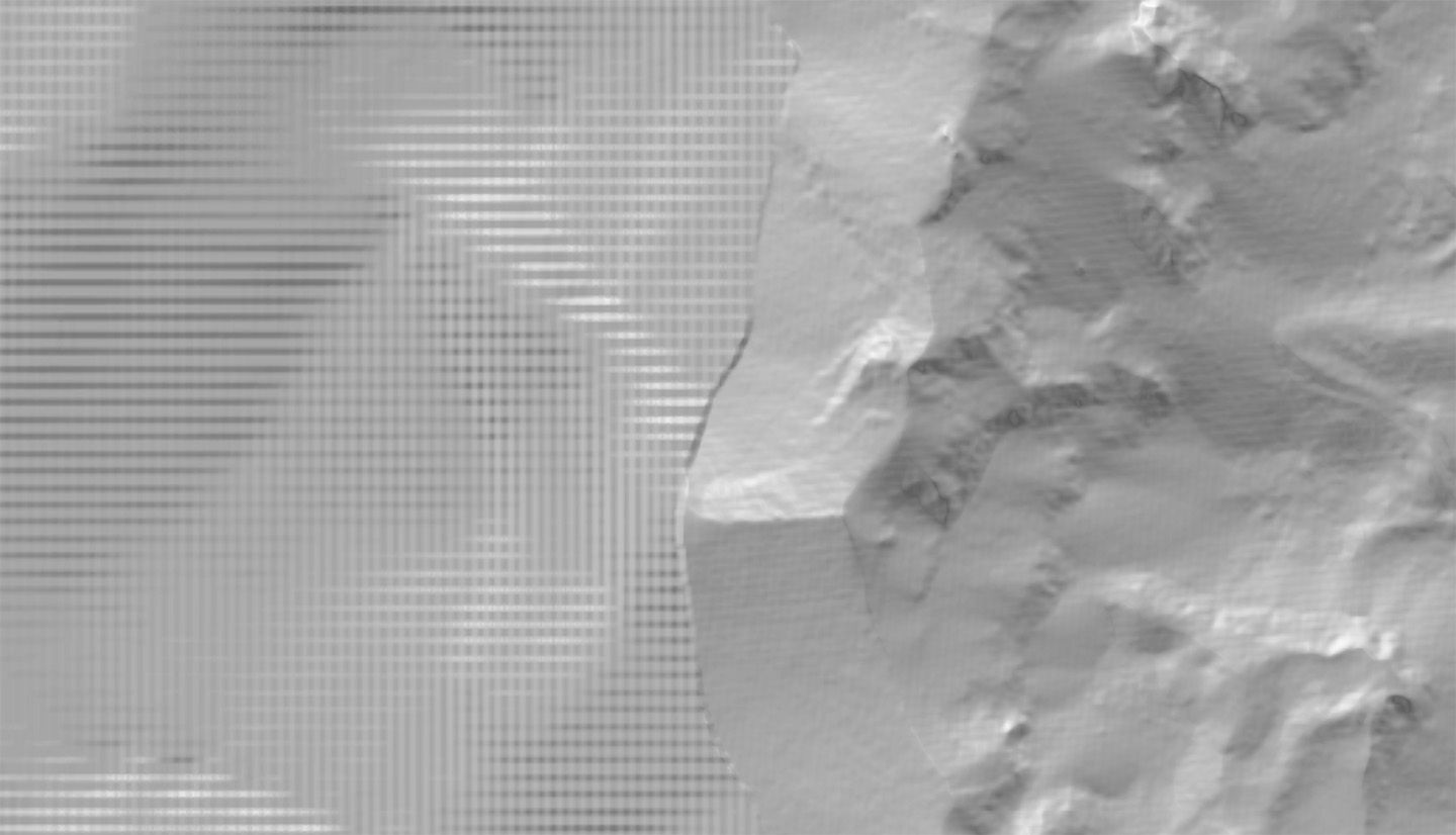
GDAL provides a variety of resampling algorithms. Here’s a comparison:

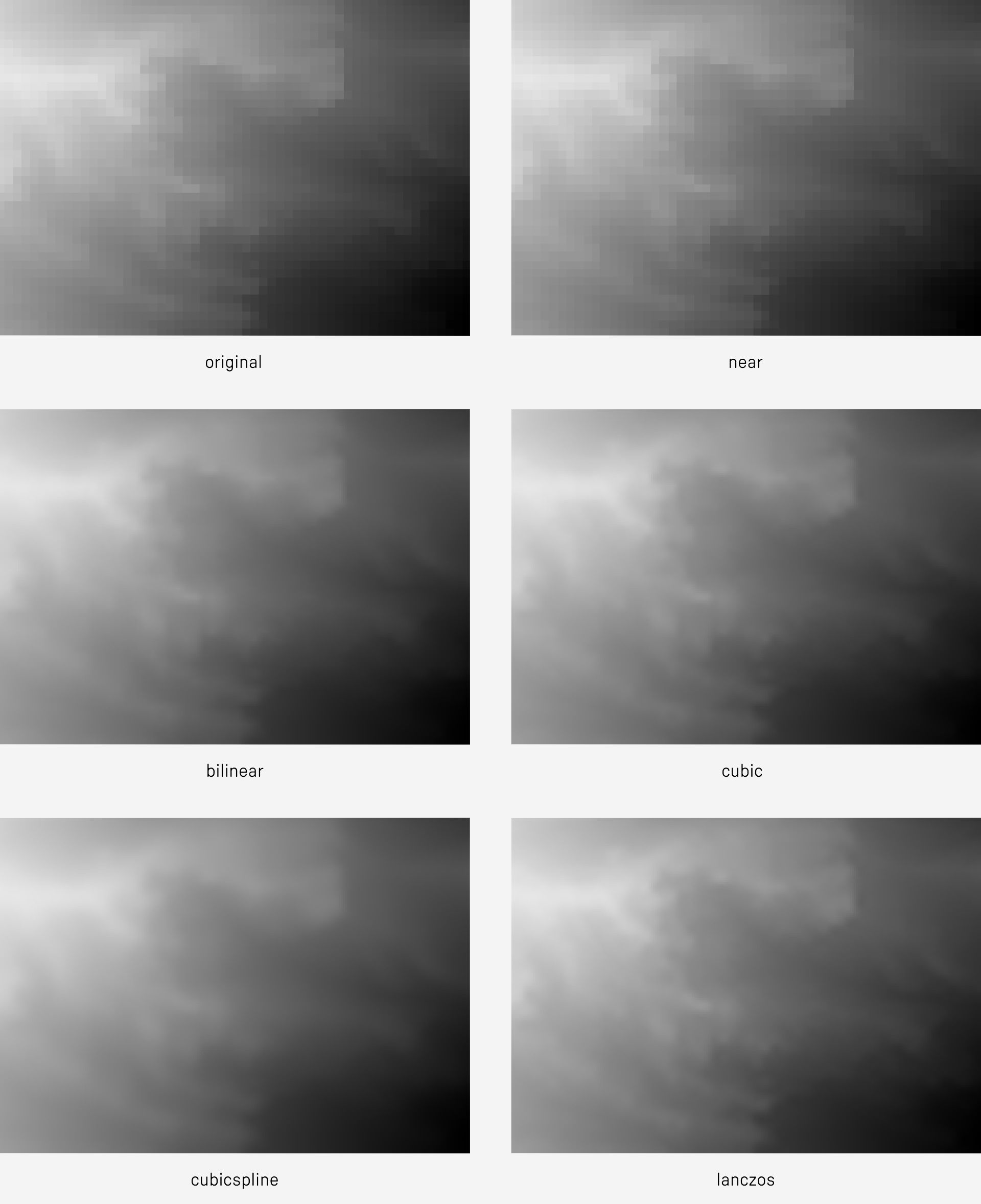
Lanczos resampling stuck out to me as it seems to bump the contrast, creating a nice looking result. This excellent stackoverflow answer explains more. Since the image represents elevation I thought it’d be best to stick to a method that’s more faithful to the original data, so I chose cubicspline. Incorporating resampling:

gdalbuildvrt \
    -overwrite \
    -vrtnodata -9999.0 \
    -resolution user \
    -tr 0.000021497547 -0.000021497547  \
    -r cubicspline \
    data/temp/dem.vrt \
    data/sources/USGS*.tif \
    data/temp/lidar.tif

Finally we regenerate the tiles, this time up to zoom level 15:

rio rgbify \
    --base-val -10000 \
    --interval 0.1 \
    --min-z 1 \
    --max-z 15 \
    --workers 10 \
    --format webp \
    data/temp/dem.vrt \
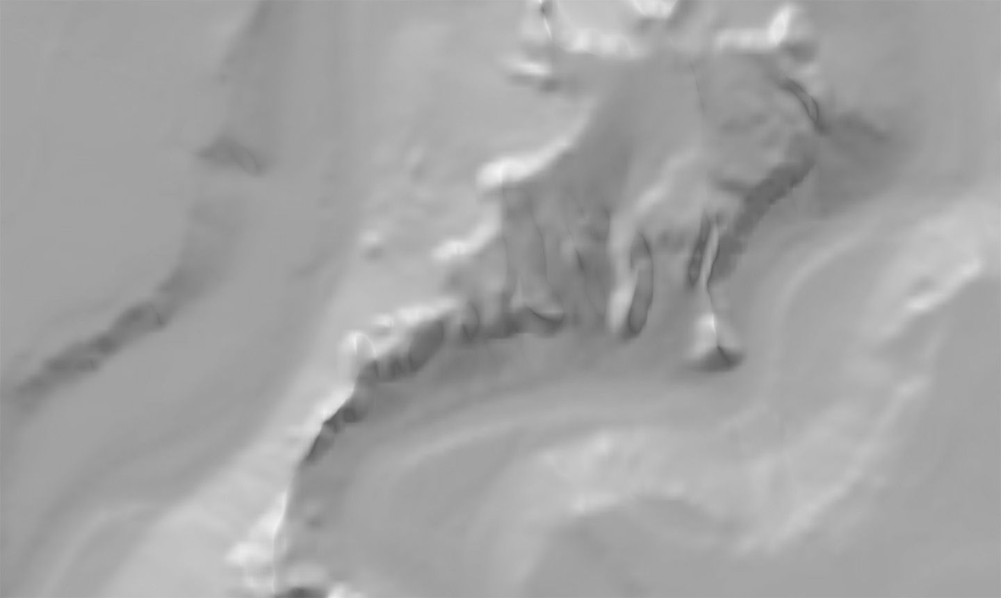
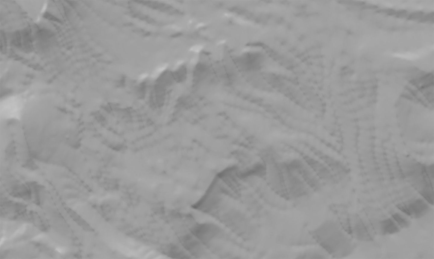
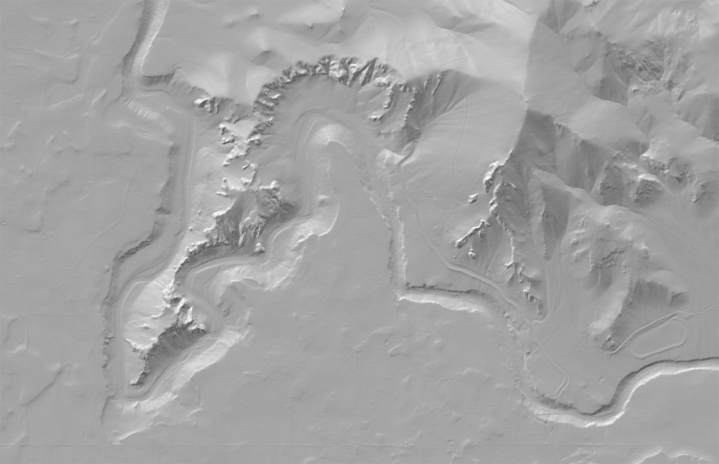
    data/output/elevation.mbtiles

Here’s the result side-by-side with the previous iteration:

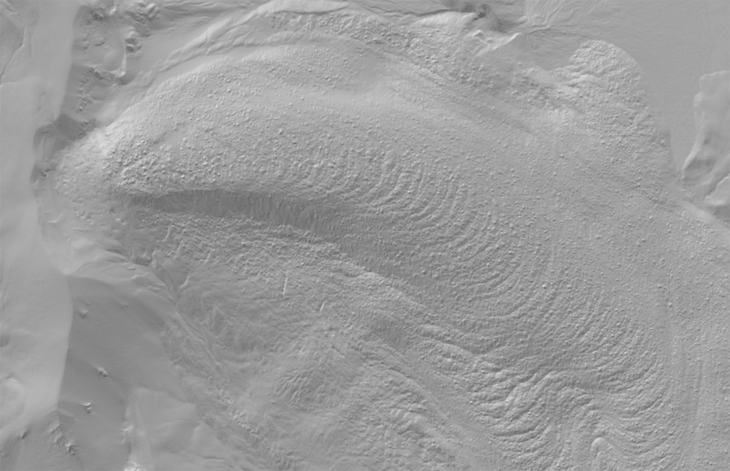
Drag to pan, double click to zoom

This resolution has plenty of detail.

Visualizing the terrain

With the tiles generated, they can be rendered with MapLibre GL JS. So far we've seen rendering the tiles in 3D, and as hillshade.

Contours

A MapLibre plugin creates contour lines on the client from the terrain tiles:

Drag to pan, double click to zoom

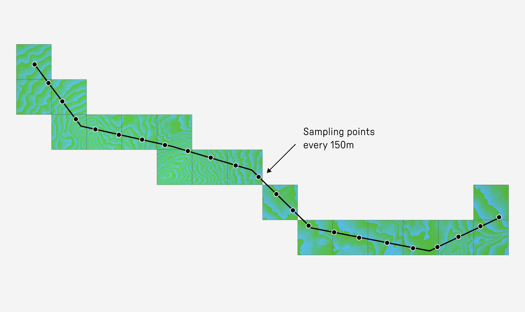
Elevation profile

Since each terrain tile contains raw elevation data, we can create elevation profiles for any line drawn on the client, such as a trail. The idea is to sample the elevation of several points on the line to create the profile.

First we'll need to fetch the elevation tiles containing each point we're sampling. The OpenStreetMap wiki describes an algorithm for determining which tile contains a specific latitude and longitude. Here's my implementation:

function getTileIndex(lng, lat, zoom) {
  const xEPSG3857 = lng
  const yEPSG3857 = Math.log(Math.tan((lat * Math.PI) / 180) + 1 / Math.cos((lat * Math.PI) / 180))
  const x = 0.5 + xEPSG3857 / 360
  const y = 0.5 - yEPSG3857 / (2 * Math.PI)
  const N = Math.pow(2, zoom)
  const xTile = N * x
  const yTile = N * y
  const xTileFractional = xTile % 1
  const yTileFractional = yTile % 1
  const xPixel = xTileFractional * 512
  const yPixel = yTileFractional * 512
  return {
    z: zoom,
    x: Math.floor(xTile),
    y: Math.floor(yTile),
    xPixel,
    yPixel,
  }
}

This gives us the tile to fetch and the x and y coordinates within to query. We can load the tile:

// get an example tile index, using maximum zoom of 15
const tile = getTileIndex(-121.79924, 44.378108, 15)
// {
//   "z": 15,
//   "x": 5297,
//   "y": 11867,
//   "xPixel": 288.00523377768695,
//   "yPixel": 47.71337864175439
// }

// fetch tile
const url = `https://<tileservice>/${tile.z}/${tile.x}/${tile.y}.webp`
const response = await fetch(url)
if (!response.ok) {
  throw new Error(`Unable to fetch elevation data for ${tile.z}/${tile.x}/${tile.y}.webp`)
}
const blob = await response.blob()

Then render it on an offscreen canvas and get the pixel value:

const bitmap = await createImageBitmap(blob)
// render in an offscreen canvas
const offscreen = new OffscreenCanvas(bitmap.width, bitmap.height)
ctx = offscreen.getContext("2d")
ctx.drawImage(bitmap, 0, 0)
// get the rgb values of the pixel we're interested in
const pixel = ctx.getImageData(tile.xPixel, tile.yPixel, 1, 1).data
const R = pixel[0]
const G = pixel[1]
const B = pixel[2]

Finally we use the formula from before to convert the TerrainRGB pixel values to an elevation:

const elevationMeters = -10000 + (R * 256 * 256 + G * 256 + B) * 0.1
const elevationFeet = elevationMeters * 3.28084

Now we can fetch the elevation for multiple points along a line. To divide the line into 150m-long sections we can use turf.js lineChunk:

const turfLine = turf.lineString(line)
const chunks = turf.lineChunk(turfLine, 150, { units: "meters" })
// get the first point of each chunk
const points = chunks.features.map((chunk) => chunk.geometry.coordinates[0])

Then fetch tiles for all the points:

// helper to fetch the elevation data for a point
const getElevation = async (point) => {
  const tile = getTileIndex(point[0], point[1], 15)
  const elevation = await getElevationTileData(tile)
  return elevation
}
// fetch elevation for all points
const responses = await Promise.allSettled(points.map((point) => getElevation(point)))

My implementation of getElevationTileData includes some caching of tiles to prevent fetching the same tile again if multiple points fall on the same tile, or if the line is moved a bit.

Here's the result:

Drag the line end points

Next: larger regions

The natural next step is to increase the size of the region. The scale is daunting though; this small example region included about 40GB of source LIDAR DEMs. For an entire state there's likely to be hundreds of gigabytes, perhaps more. I'll need to adjust the method to take this into account. I'll also need a better computer.

⁂